A lot of machine learning problems in the real world suffer from the curse of dimensionality; you’ve got fewer training instances than you’d like, and predictive signal is distributed (often unpredictably!) across many different features. Sometimes when your target is continuously-valued, there simply aren’t enough instances to predict these values to the precision of regression. In this case, we can sometimes transform the regression problem into a classification problem by binning the continuous values into makeshift classes. But how do we pick the bins? In this post, I’ll walk through a case study, starting with a naive approach and moving to a more informed strategy using the visual diagnostics library Yellowbrick.
Dataset Intro
I’ve been doing a lot of work on text analysis lately, and was looking for novel corpora that could be used for sentiment analysis. In college, I was lucky enough to be friends with a few cool people like Jayson Greene who ended up working at the music review website https://pitchfork.com/. Pitchfork is kind of notorious for having incredibly detailed and often hilariously snarky reviews of newly released albums. For example, here’s an excerpt from Jayson’s review of Maroon 5’s newest album:
“Adam Levine’s voice is one of the most benignly ubiquitous sounds in pop. It is air-conditioning, it is tap water, it is a thermostat set to 72 degrees…It’s this utter lack of libido that ends up making Red Pill Blues so difficult to even finish.”
Each review has a score between 0 and 10 (this one got a 4.8). I was curious about whether it might be possible to predict the score assigned to an album based on the bag-of-words of the text.
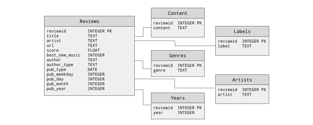
There’s a Kaggle dataset that includes about 18K historic reviews, which I found here. The data is stored in a sqlite database with the following schema:

Since text is very high dimensional, I knew that it would be unlikely that I’d be able to use regression to predict the floating point score of the review. Instead I decided I’d attempt to bin the scores into 4 ranges roughly corresponding to sentiment (e.g. “terrible”, “okay”, “great”, and “amazing”). In the next section, I’ll show the text preprocessing work I did in advance of classification, but if you aren’t planning to run this code yourself, feel free to skip it and go straight to Creating the Bins for the Pipeline.
Preparing the Data
To prepare the data for sentiment analysis, I started by writing a custom corpus reader that would give me streaming access to each of the reviews, including the score, the album name, the artist, and the text:
import sqlite3


class SqliteCorpusReader(object):
    """
    Provides streaming access to sqlite database records
    """
    def __init__(self, path):
        self._cur = sqlite3.connect(path).cursor()

    def scores_albums_artists_texts(self):
        """
        Returns a generator with each review represented as a
        (score, album name, artist name, review text) tuple
        """
        sql = """
              SELECT S.score, L.label, A.artist, R.content
              FROM [reviews] S
              JOIN labels L ON S.reviewid=L.reviewid
              JOIN artists A on L.reviewid=A.reviewid
              JOIN content R ON A.reviewid=R.reviewid
              """
        self._cur.execute(sql)
        for score,album,band,text in iter(self._cur.fetchone, None):
            yield (score,album,band,text)
Next I created a custom preprocessor class to tokenize and part-of-speech tag the reviews, and store the transformed corpus to a new directory:
import os
import nltk
import pickle
from slugify import slugify


class Preprocessor(object):
    """
    The preprocessor wraps a SqliteCorpusReader and manages the stateful
    tokenization and part of speech tagging into a directory that is stored
    in a format that can be read by the `PickledCorpusReader`. This format
    is more compact and necessarily removes a variety of fields from the
    document that are stored in Sqlite database. This format however is more
    easily accessed for common parsing activity.
    """
    def __init__(self, corpus, target=None, **kwargs):
        """
        The corpus is the `SqliteCorpusReader` to preprocess and pickle.
        The target is the directory on disk to output the pickled corpus to.
        """
        self.corpus = corpus
        self.target = target

    @property
    def target(self):
        return self._target

    @target.setter
    def target(self, path):
        if path is not None:
            # Normalize the path and make it absolute
            path = os.path.expanduser(path)
            path = os.path.expandvars(path)
            path = os.path.abspath(path)

            if os.path.exists(path):
                if not os.path.isdir(path):
                    raise ValueError(
                        "Please supply a directory to write preprocessed data to."
                    )

        self._target = path

    def abspath(self, name):
        """
        Returns the absolute path to the target fileid from the corpus fileid.
        """
        # Create the pickle file extension
        fname  = str(name) + '.pickle'

        # Return the path to the file relative to the target.
        return os.path.normpath(os.path.join(self.target, fname))

    def tokenize(self, text):
        """
        Segments, tokenizes, and tags a document in the corpus. Returns a
        generator of paragraphs, which are lists of sentences, which in turn
        are lists of part of speech tagged words.
        """
        yield [
            nltk.pos_tag(nltk.wordpunct_tokenize(sent))
            for sent in nltk.sent_tokenize(text)
        ]

    def process(self, score_album_artist_text):
        """
        For a single file does the following preprocessing work:
            1. Checks the location on disk to make sure no errors occur.
            2. Gets all paragraphs for the given text.
            3. Segments the paragraphs with the sent_tokenizer
            4. Tokenizes the sentences with the wordpunct_tokenizer
            5. Tags the sentences using the default pos_tagger
            6. Writes the document as a pickle to the target location.
        This method is called multiple times from the transform runner.
        """
        score, album, artist, text = score_album_artist_text

        # Compute the outpath to write the file to.
        if album:
            name = album+'-'+artist
        else:
            name = artist
        target = self.abspath(slugify(name))
        parent = os.path.dirname(target)

        # Make sure the directory exists
        if not os.path.exists(parent):
            os.makedirs(parent)

        # Make sure that the parent is a directory and not a file
        if not os.path.isdir(parent):
            raise ValueError(
                "Please supply a directory to write preprocessed data to."
            )

        # Create a data structure for the pickle
        document = list(self.tokenize(text))
        document.append(score)

        # Open and serialize the pickle to disk
        with open(target, 'wb') as f:
            pickle.dump(document, f, pickle.HIGHEST_PROTOCOL)

        # Clean up the document
        del document

        # Return the target fileid
        return target

    def transform(self):
        """
        Transform the wrapped corpus, writing out the segmented, tokenized,
        and part of speech tagged corpus as a pickle to the target directory.
        This method will also directly copy files that are in the corpus.root
        directory that are not matched by the corpus.fileids().
        """
        # Make the target directory if it doesn't already exist
        if not os.path.exists(self.target):
            os.makedirs(self.target)

        for score_album_artist_text in self.corpus.scores_albums_artists_texts():
            yield self.process(score_album_artist_text)
After using the transform method to convert the raw corpus into a preprocessed corpus, I added a second corpus reader that would be able to stream the processed documents:
import pickle
from nltk.corpus.reader.api import CorpusReader

PKL_PATTERN = r'(?!\.)[\w\s\d\-]+\.pickle'


class PickledReviewsReader(CorpusReader):
    def __init__(self, root, fileids=PKL_PATTERN, **kwargs):
        """
        Initialize the corpus reader
        """
        CorpusReader.__init__(self, root, fileids, **kwargs)

    def texts_scores(self, fileids=None):
        """
        Returns the document loaded from a pickled object for every file in
        the corpus. Similar to the SqliteCorpusReader, this uses a generator
        to achieve memory safe iteration.
        """
        for path, enc, fileid in self.abspaths(fileids, True, True):
            with open(path, 'rb') as f:
                yield pickle.load(f)

    def reviews(self, fileids=None):
        """
        Returns a generator of paragraphs where each paragraph is a list of
        sentences, which is in turn a list of (token, tag) tuples.
        """
        for text,score in self.texts_scores(fileids):
            yield text

    def scores(self, fileids=None):
        """
        Returns a generator of scores
        """
        for text,score in self.texts_scores(fileids):
            yield score
Next I added a custom class to lemmatize and remove stop words:
import unicodedata
from nltk.corpus import wordnet as wn
from nltk.stem.wordnet import WordNetLemmatizer
from sklearn.base import BaseEstimator, TransformerMixin

class TextNormalizer(BaseEstimator, TransformerMixin):

    def __init__(self, language='english'):
        self.stopwords  = set(nltk.corpus.stopwords.words(language))
        self.lemmatizer = WordNetLemmatizer()

    def is_punct(self, token):
        return all(
            unicodedata.category(char).startswith('P') for char in token
        )

    def is_stopword(self, token):
        return token.lower() in self.stopwords

    def normalize(self, document):
        return [
            self.lemmatize(token, tag).lower()
            for sentence in document
            for (token, tag) in sentence
            if not self.is_punct(token)
               and not self.is_stopword(token)
        ]

    def lemmatize(self, token, pos_tag):
        tag = {
            'N': wn.NOUN,
            'V': wn.VERB,
            'R': wn.ADV,
            'J': wn.ADJ
        }.get(pos_tag[0], wn.NOUN)

        return self.lemmatizer.lemmatize(token, tag)

    def fit(self, documents, y=None):
        return self

    def transform(self, documents):
        return [
            ' '.join(self.normalize(doc)) for doc in documents
        ]
Creating the Bins for the Pipeline
Ok, now it’s time to bin the continuous target values of the reviews into buckets for classification. I did this using NumPy’s digitize method, naively partitioning the score range into evenly spaced quartiles:
import numpy as np

def documents(corpus):
    """
    This will give us access to our features (X)
    """
    return list(corpus.reviews())

def continuous(corpus):
    """
    This will give us access to our continuous targets (y)
    """
    return list(corpus.scores())

def categorical(corpus):
    """
    This will give us access to our binned targets (y):
    terrible : 0.0 < y <= 3.0
    okay     : 3.0 < y <= 5.0
    great    : 5.0 < y <= 7.0
    amazing  : 7.0 < y < 10.1
    """
    return np.digitize(continuous(corpus), [0.0, 3.0, 5.0, 7.0, 10.1])
Preliminary Text Analytics Pipeline
We can now use a Scikit-Learn pipeline to chain our transformation, vectorization, and classification steps together, as follows:
if __name__ == '__main__':
    from sklearn.pipeline import Pipeline
    from sklearn.neural_network import MLPClassifier
    from sklearn.model_selection import cross_val_score
    from sklearn.feature_extraction.text import TfidfVectorizer

    corpus_path = '../processed_review_corpus'

    pipeline = Pipeline([
        ('normalize', TextNormalizer()),
        ('vectorize', TfidfVectorizer()),
        ('classify', MLPClassifier(hidden_layer_sizes=[50,15], verbose=True))
    ])

    corpus = PickledReviewsReader(corpus_path)
    X = documents(corpus)
    y = categorical(corpus)
    scores = cross_val_score(pipeline, X, y, cv=12) #may take a while!
0.71
A mean score of 0.71 is ok, but nothing to write home about. The next step is to try to figure out why the score isn’t great – it could be a number of things, including:
- the hyperparameters we’ve selected for our model,
MLPClassifier, are the optimal ones MLPClassifierisn’t the best choice of model for the job- our
TextNormalizer, which performs dimensionality reduction through lemmatization, is not reducing the dimensionality enough - there simply isn’t enough signal in the data
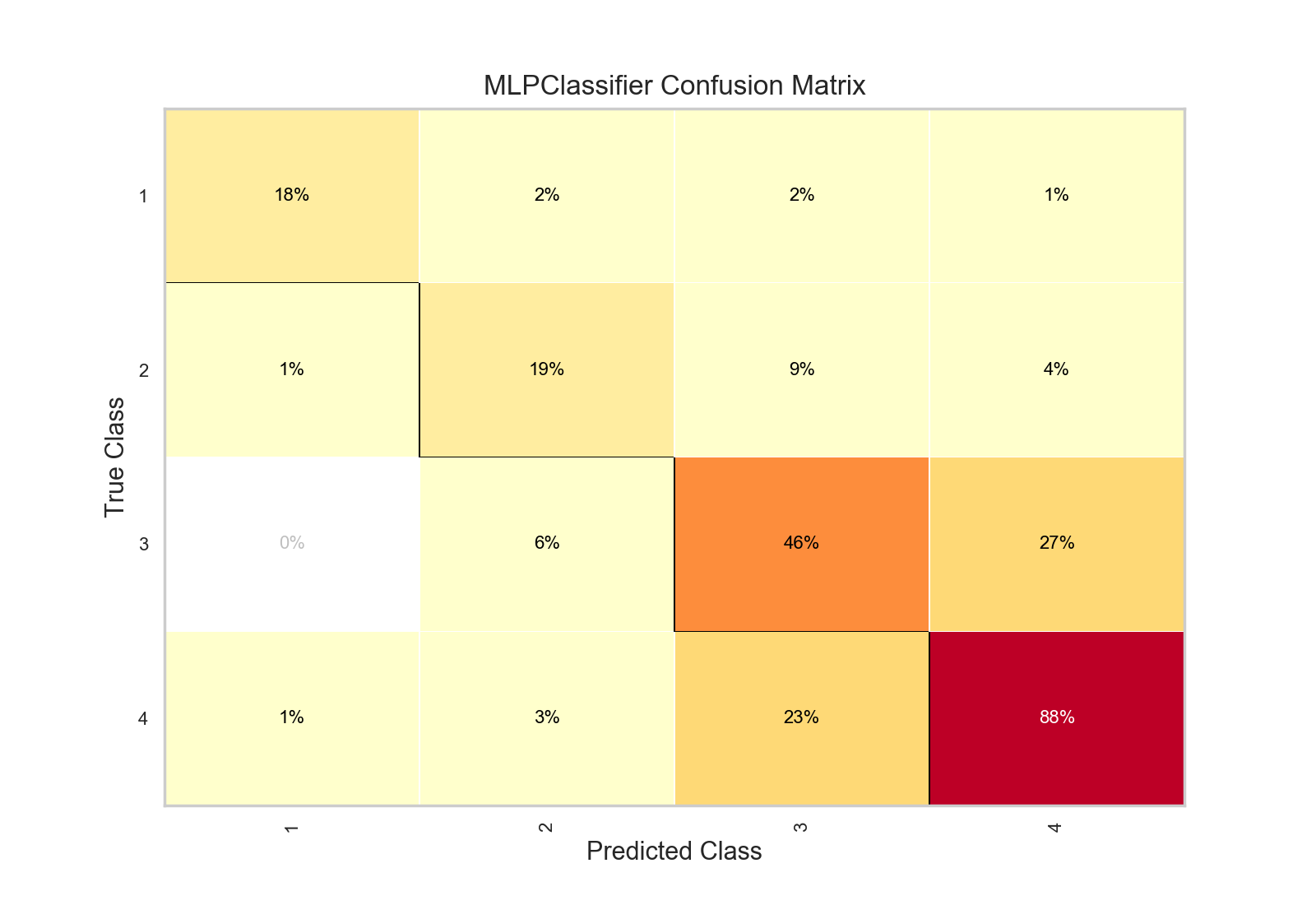
Let’s use Yellowbrick’s ConfusionMatrix to visually evaluate to see if we can diagnose what’s happening when our classifier tries to predict which reviews correspond to the four different bins of scores:
from yellowbrick.classifier import ConfusionMatrix
from sklearn.model_selection import train_test_split as tts

X_train, X_test, y_train, y_test = tts(X, y, test_size=0.4)
cm = ConfusionMatrix(pipeline)
cm.fit(X_train, y_train)
cm.score(X_test, y_test)
cm.poof()

The ConfusionMatrix takes a fitted Scikit-Learn classifier and a set of test X and y values and returns a report showing how the test values’ predicted classes compare to their actual classes. The idea is that it’s supposed to tell you where your classifier is getting mixed up. As such, they certainly provide more information than top-level scores, but I always find them a bit difficult to unpack, particularly the more classes I have.
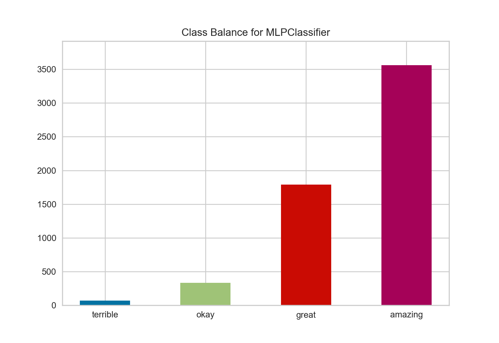
Yellowbrick’s ClassBalance, which is a bit simpler, enables us to get the break down between the four classes:
from yellowbrick.classifier import ClassBalance

target_names = ["terrible", "okay", "great", "amazing"]
cb = ClassBalance(pipeline, classes=target_names)
cb.fit(X_train, y_train)
cb.score(X_test, y_test)
cb.poof()

Ah - there’s my problem. I have a massive class imbalance. Under the binning scheme I used, there simply aren’t enough “terrible” and “okay” albums for my classifier to learn on. It’s unlikely to ever really predict much other than “amazing”.
My binning strategy was admittedly a bit naive, and I made an assumption that the reviews would be pretty much evenly distributed across the four bins. Boy was I wrong! This is a clear case of selection bias – my assumption was based on my vivid memories of all of the hilariously dissed and panned albums, when of course most Pitchfork reviewers are probably going to be listening to and reviewing good or very good albums. The low-scoring ones, while memorable, are relatively few.
Conclusion
What if there was a way to combine the insight from ConfusionMatrix with the interpretability of ClassBalance? My friend recently sent me some prototype code that looks very promising!
import numpy as np
import matplotlib.pyplot as plt

from matplotlib import cm
from sklearn.utils.multiclass import unique_labels
from sklearn.metrics.classification import _check_targets


def plot_class_balance_preds(y_true, y_pred, labels=None, ax=None):
    # Use Sklearn tools to validate the target
    # Note y_true and y_pred should already be label encoded
    y_type, y_true, y_pred = _check_targets(y_true, y_pred)
    indices = unique_labels(y_true, y_pred)

    # Create a 2D numpy array where each row is the count of
    # the predicted classes and each column is the true class
    data = np.array([
        [(y_pred[y_true==label_t] == label_p).sum() for label_p in indices]
        for label_t in indices
    ])

    # Ensure that the number of elements in data matches y_pred and y_true
    # Not necessary but used as a sanity check
    assert data.sum() == len(y_pred) == len(y_true)

    # labels_present is the indices of the classes, labels is the string names
    # Another sanity check, this will not prevent missing classes, which is bad
    labels = labels if labels is not None else indices
    assert len(labels) == len(indices)

    # Create a matplotlib axis
    if ax is None:
        _, ax = plt.subplots()

    # Create a unique color for each predict class
    colors = [cm.spectral(x) for x in np.linspace(0, 1, len(indices))]

    # Track the stack of the bar graph
    prev = np.zeros(len(labels))

    # Plot each row
    for idx, row in enumerate(data):
        ax.bar(indices, row, label=labels[idx], bottom=prev, color=colors[idx])
        prev += row

    # Make the graph pretty
    ax.set_xticks(indices)
    ax.set_xticklabels(labels)
    ax.set_xlabel("actual class")
    ax.set_ylabel("number of predicted class")

    # Put the legend outside of the graph
    plt.legend(bbox_to_anchor=(1.04,0.5), loc="center left")
    plt.tight_layout(rect=[0,0,0.85,1])

    return ax
So now, when we use the plot_class_balance_preds method:
X_train, X_test, y_train, y_true = tts(X, y, test_size=0.33)
pipeline.fit(X_train, y_train)
y_pred = pipeline.predict(X_test)
g = plot_class_balance_preds(y_true, y_pred, labels=target_names)
plt.show()
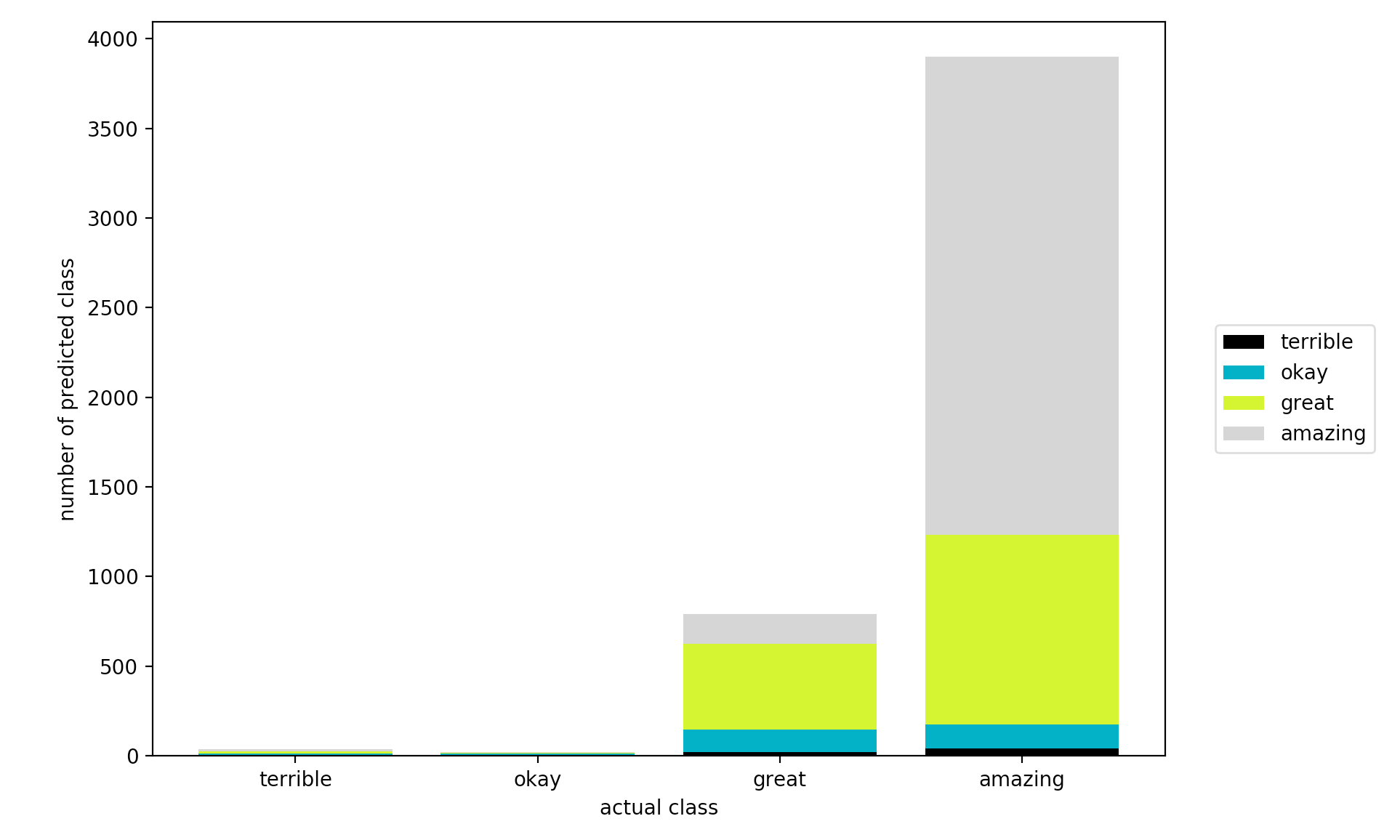
We get this:

How fascinating! I find this bar chart incredibly easy to read. It’s essentially telling me that when my classifier guesses an album is “amazing”, it’s usually right. The model also learns that if an album isn’t “amazing”, it’s most likely “great”. In terms of error, it equally gets “okay” and “amazing” wrong.
I thought it would be awesome if someone would pull this into Yellowbrick, and it looks like it’s already in the works. There’s even a prototype for a balanced binning visualizer!
